Are Spectral Risk Measures Respectable Enough?
Spectral risk measures are relatively new entrants to the field of risk management, with the distinctive feature that they relate the risk measure directly to the user’s risk aversion function. This post discusses the pros and cons of using them from a practical “real world” perspective.
Whenever I work with risk measures, or any other quantitative model for that matter, I am reminded of a Calvin and Hobbes comic strip where Calvin argues, quite convincingly, that math is not a science but a religion. To quote him: “All these equations are like miracles. You take two numbers and when you add them, they magically become one NEW number! No one can say how it happens. You either believe it or you don’t. This whole book is full of things that have to be accepted on faith! It’s a RELIGION!”
I guess one can make a similar argument about risk measures. You either believe them or you don’t! Before we pass judgment on the believability of these measures, however, we need to have some reasonable, logical basis for evaluating them.
First, let’s take a minute to ponder what a risk measure is all about. From an existential perspective, the sole purpose of a risk measure is to quantify the uncertainty associated with an expected payoff (say, of an asset or a portfolio) at some point in the future. Mathematically speaking, if we consider a portfolio payoff as a random variable, then we can apply some function to it to come up with a risk measure. For instance, the historical volatility of a portfolio is nothing but the standard deviation of the portfolio returns measured at a certain frequency over a certain time period.
As a start, for risk measures to be considered “respectable,” they have to be, at the very least, “coherent.” For risk measures to be considered coherent, Artzner et al. espouse (PDF) that they exhibit the following properties:
- monotonicity,
- sub-additivity,
- positive homogeneity, and
- translational invariance.
To explain this notion, let’s assume that X and Y represent two portfolios and that Q(.) is a measure of risk over a given time horizon.
The monotonicity axiom requires that if portfolio X always has smaller losses than portfolio Y (or put another way, portfolio X always has better values than portfolio Y), then the risk measure of portfolio X should be less than that of portfolio Y. So, for all X,Y 


A simple example would be where both X and Y are call options on the same stock, with X having a lower strike price than Y.
The sub-additivity axiom fleshes out the concept of diversification. It requires that, because of correlation benefits, the combined risk of two assets be less than or equal to the sum of risks of the individual assets. The entire concept of portfolio construction relies on this key notion. Sub-additivity can be expressed as Q(X+Y) 
Positive homogeneity satisfies the relation Q(λX) = λQ(X), where λ is greater than 0. This implies that when wealth under risk is multiplied by a positive factor, the associated risk must also grow with the same proportionality. So, if you double the assets under risk, the risk doubles too.
A risk measure is said to display convexity when it has both sub-additivity and positive homogeneity. Convexity plays a very important role in statistics and is a desirable characteristic, especially in portfolio optimization, because it assures us that an optimal solution will be found.
Translational invariance refers to the fact that risk is unaffected by the addition or removal of a certain amount of riskless capital. Translational invariance is represented by the equation Q(X + c) = Q(X) + c, where c is the riskless capital under consideration.
How Do Value at Risk (VaR) and Expected Shortfall (ES) Measure Up On the “Coherence” Scale?
Two of the most frequently used tail risk measures are VaR and ES. One of the biggest issues with VaR is that it does not satisfy the properties of coherence, sub-additivity in particular. The aggregate VaR for the portfolio can be greater than the summed VaR of each individual security in the portfolio.
The other obvious issue is the fact that it does not reveal anything about the magnitude of losses exceeding the VaR limit. Unfortunately, even using a high confidence level does not mitigate these critical issues. However, using a bounded solution, such as conditional value at risk, resolves them both.
In the case of a continuous loss distribution, ES is given by

where q is the quantile of the loss distribution for a given tail probability p; ES is the average of the worst 100(1 – α)% of losses, where α is the confidence level.
At first glance, ES seems to be a perfect alternative to VaR. Unlike VaR, ES is coherent and has many of the properties one would desire in a “respectable” risk measure. ES also takes into account the magnitude of losses that exceed VaR. Hence, the ES measure appears to provide a better basis for estimating risk than does VaR.
But the ES measure runs into one small problem. Using an ES measure implies that only losses beyond the tail limit are taken into account whereas those that are below it are disregarded. Also, ES gives all losses beyond the tail limit an equal weight, which is inconsistent with risk aversion because it suggests that with respect to outcomes beyond the tail limit, one is risk neutral between better and worse outcomes. Moreover, the user still has the problem of determining what the tail probability, p, should be.
What are Spectral Risk Measures and Why Do We Need Them?
Spectral risk measures (SRMs) enable us to overcome this latter problem. They are also coherent and have the advantage that they alone take into account the user’s degree of risk aversion. Simply put, SRM is a risk measure that is calculated as a weighted average of outcomes, the weights of which depend on the user’s risk aversion.
Mathematically, SRM can be defined as (
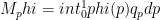
for some weighting function 
Spectral risk measures thus enable us to associate the risk measure with the user’s attitude toward risk. Therefore, we might expect that, all else being equal, if a user is more risk averse, then that user should face a higher risk, as given by the value of the SRM.
SRMs can be applied to many different problems. Studies have suggested using them to set capital requirements, to obtain optimal risk-expected return tradeoffs, or even to set margin requirements for futures clearinghouses.
Issues with SRMs
To obtain a spectral risk measure, users must specify a particular form for their risk aversion function. Most of the relevant studies discuss using the exponential utility function to reflect the user’s absolute risk aversion. Whether the exponential utility function provides a good description of “real world” risk aversion is debatable.
The exponential utility function implies that the coefficient of absolute risk aversion is constant and that the coefficient of relative risk aversion increases with wealth. This notion goes against the real-world empirical observation of decreasing risk aversion because risk appetite usually increases with increasing wealth, whereas there is no direct connection between observable risk premiums and the level of wealth. Thus, the absolute and relative risk aversion properties of the exponential utility function do not match what is generally observed in the real world.
Unfortunately, the literature gives very little guidance on the appropriate choice of risk aversion function or how one might go about choosing it. The general lesson is that users of spectral risk measures must be careful to ensure that they pick utility functions that fit the features of the particular problems they are dealing with.
If you liked this post, don’t forget to subscribe to the Enterprising Investor.
All posts are the opinion of the author. As such, they should not be construed as investment advice, nor do the opinions expressed necessarily reflect the views of CFA Institute or the author’s employer.